The contents of this blog post are inherited from a short research project by Group 10 of the Information Retrieval and Data Mining module at University College London. Instead of letting it rot in my Dropbox, I decide to free the knowledge and hope someone finds it useful.
The research goal was to predict stock market performance of companies listed on Dow Jones Industrial Average using Twitter Sentiment Analysis. I’ll be honest, the prediction part wasn’t as awesome as we expected it to be, but the rest is fine, and fun to read through.
Abstract
Modern data mining techniques have given birth to the rise of sentiment analysis, an algorithmic approach towards detecting sentiment of a product or company using social media data. A popular use case of sentiment analysis has been stock market predictions, which, for finance aficionados, has remained a very powerful tool for analysis.
During the course of this report, we aim to showcase various techniques that are able to derive sentiment from a large Twitter dataset, consisting of companies listed on Dow Jones Industrial Average. To limit the scope of our research, we are dealing with 3 companies listed on DJIA, namely American Express (Amex), Boeing and AT&T.
We have experiment with various sentiment analysis techniques, from sentiment lexicon-driven approaches to multinomial regression techniques, and have derived sentiment polarities of each tweet, with respect to the pre-processed dataset of the 3 companies. Furthermore, we have attempted to form correlations of our sentiment analysis with real DJIA data.
The results are resounding, such that that sentiment lexicon-driven techniques were able to detect sentiment polarity that correlate highly with real Y! Finance stock data. We have shown that the strength of our algorithms (combined with solid pre-processing policies) also detected events like the 2nd February 2014 “Superbowl”. The plot charts contained in the report clearly demonstrate this with overlays of sentiment graphs and real stock data.
Our multinomial regression technique based on logistical regression has also shown resounding success. We were able to predict the right sentiment more than 83% of the time. Please see the code files in the .zip that accompany the report. We have included code snippets in this report where necessary.
1. Introduction
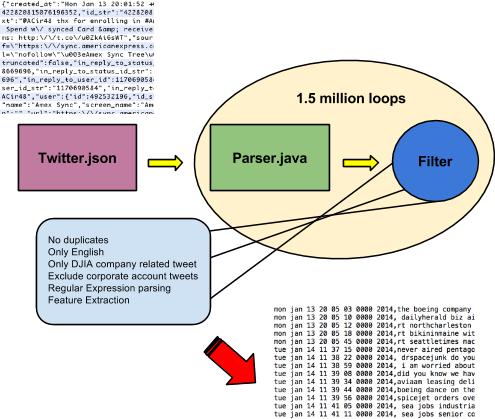
We have access to a larger than 5GB dataset which was obtained from Twitter by a university associate using the Twitter Streaming API. The screenshot below shows the content of the text file in JSON format. This requires a great amount of pre-processing to ensure the following points are satisfied.
2. Pre-Processing Policies
- Only features that are necessary will be extracted using a JSON parser.
- Removal of junk, i.e. tweets not related to DJIA listed companies.
- Ensuring tweets by the companies themselves are omitted.
- Creation of 3 sub-datasets for each, Boeing, AT&T and American Express (Amex).
- Ensure all tweets are in the “English language”.
- Remove duplicate tweets using a LinkedHashSet.
The pre-processing steps are outlined in the next sections briefly to display how it was carried out, as it forms a crucial part of the first step towards sentiment analysis.
2.1 Parsing JSON
Twitter data is stored in a JSON format, a lightweight technology used for data marshalling. For processing of over 5GB of JSON data, we used a Java library called JSON Simple[5]. JSON Simple easily allows parsing of JSON objects with great ease, as demonstrated below. Before we proceed further, it is worthwhile looking at the JSON object that ships with the dataset. This is a Twitter Streaming API standard.
2.1.1 The JSON Object
This is a snippet of the top level JSON object which contains many pieces of information.
Key parts to parse from this object are:
- “created_at” : string which ensures we keep track of the period of tweet
- “text” : string which is essentially the crux of the matter, the tweet itself.
- “lang” : string to ensure we only get English tweets.
From the {}user array, it is worthwhile parsing the following information:
- “name”
- “followers_count”
- “statuses_count”
We are not extracting hashtags and their respective arrays primarily because the hashtags are themselves part of the tweet.
2.2. The Actual Parsing
The Parser.java file contains the code for performing graceful parsing of the tweets for our sentiment analysis. The parser works accurately and spits out the text in the form below. Note, the .equals() was set to “mcdonalds” for this sample.
As you can see, the format of the parsed tweet is fairly straightforward to understand. Recall that the hashtags and indices have been excluded, as the hashtag itself is parsed into the tweet directly during extraction. This is the data we are playing with:
Date, Tweet, Language, Name, Followers, Tweets
The process of parsing a Twitter dataset is a crucial part of any sentiment analysis undertaking and it is worthwhile mentioning the programmatic process used to glean and clean the data.
Parser.java
This section shows a few snippets to demonstrate the process that was carried out for pre-processing Twitter streaming data for sentiment analysis.
Parsing lines into JSON Object
//parse each line into an Object
Object obj = parser.parse(line);
JSONObject jsonObject = (JSONObject) obj;

//get the created date
String created_at = (String) jsonObject.get("created_at");
sb.append(created_at+",");

//get the tweet
String tweet = ((String) jsonObject.get("text"));
String mod = tweet.replaceAll(",", "");
The Filtering Core
//Filtering for the DJIA listed company
if ( ( (processed_string.indexOf( "amex" ) > -1) || (processed_string.indexOf( "americanexpress" ) > -1) || (processed_string.indexOf( "american express" ) > -1) ) && (processed_string.endsWith(",")) ) {
//break it into pieces for matching
String [] sp = processed_string.split(",");
String tweet_f = sp[1];
String lang_f = sp[2];
String user_f = sp[3];
//add .replace("at& t","at&t") if using for AT&T
String final_f = processed_string.substring(0, processed_string.length() - 1);
//only English tweets and non duplicates and not from companies
if ((lang_f.equals("en")) && !(user_f.equals(amex)) && !(ln.contains(tweet_f)) ) {
bw.write(final_f+"\n");
count_processed++;
}
//register tweet in LinkedHashSet and track
ln.add(tweet_f);
}
Regex Filter
//keep &, symbol for AT&T and separators
String processed_string = sb.toString().toLowerCase().replaceAll("[^A-Za-z0-9^&,']+"," ");
System.out.println(count);

//remove URL
String mod_no_url = mod.replaceAll("https?://\\S+\\s?", "");
sb.append(mod_no_url+",");
Order of Tweets
A considerable amount of thought was put into ensuring the order of tweets are maintained (time, stocks), and that there are no duplicates, which might pose threats to the accuracy of sentiment calculation. For this purpose, a LinkedHashSet was utilized, which maintains insertion order and removes duplicates, as a Set would.
//duplicate tweets removal
LinkedHashSet<String> ln = new LinkedHashSet<String>();
3. Sentiment Analysis
Once we successfully pre-processed the data, there were ample set of data points to play with, which are described in the diagram below. The subsequent sections will highlight the different techniques to reveal sentiment within these tweets.
However, there is a considerable amount of junk within the tweets themselves, like stop words. An appropriate stop word dictionary will accompany the sentiment algorithm to leave only the important words for polarity detection.
Removal of Stopwords
Stopwords are considered useless because they add a considerable amount of unnecessary weightage to the bag of words, increasing index size and time. A popular stopwords.txt corpus has been obtained from Google Code repository [1] that will be utilized to filter our pre-processed dataset.
StopWordsFilter.java
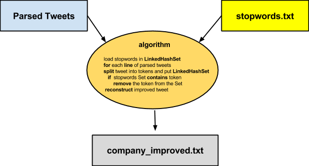
The above image shows the StopWordsFilter.java at work. For example, in amex.txt (containing American Express tweets), 54,777 tweets were filtered and 206,629 stop words were removed. Here’s a brief overview of the mechanics of the stop words filter. Also, since a Set has been used, tweets do not have duplicate words in them anymore.
The section below describes the core algorithm in Java that was used to perform the stop words filtering. The algorithm is efficient and uses .setLength(0) to flush the StringBuilder every time a new tweet is encountered.
while ((line = br.readLine()) != null) {
//store tweet splits
LinkedHashSet<String> tweets  = new LinkedHashSet<String>();
//We need to extract tweet and their constituent words
String [] tweet = line.split(",",3);
String input =tweet[1];
String [] constituent = input.split(" ");
//add all tokens in set
for (String a : constituent) {
tweets.add(a.trim());
}
LinkedHashSet<String> tweets_set  = new LinkedHashSet<String>(tweets);
System.out.println("Before: "+tweets);
//replace stopword
for (String word : tweets_set) {
if (stopwords.contains(word)) {
tweets.remove(word);
stop_word_count++;
}
}
//re build the tweet after stop word removal
for (String t : tweets) {
sb.append(t+" ");
}
//String Builder Let's Do it.
String stop_word_less_tweet = sb.toString();
System.out.println("After: "+stop_word_less_tweet);
String result = tweet[0] + "," + stop_word_less_tweet + "," + tweet[2];
System.out.println(result);
bw.write(result+"\n");
count_processed++;
//flush StringBuilder
sb.setLength(0);
}
3.1 Sentiment Analysis using Lexicon Approach
Sentiment Lexicons are datasets containing positive and negative words, often with their polarity scores, but often by themselves. In this section, we will explore our first technique for sentiment analysis. A popular approach, it works accurately if amalgamated with more advanced NLP techniques.
Bing Liu[2] (2004) has made available a 6800 word sentiment word dataset without polarity scores. We will now perform sentiment analysis for the 3 DJIA companies using this dataset. We will look into more advanced lexicons later, as you will see. The goal of this section is to demonstrate a working sentiment analysis algorithm.
Sentiment Lexicon
The two images above show a screenshot of our sentiment lexicon. Since there is no polarity associated with any of the tokens, a negative word = -1 and a positive word = 1. This is to ensure that a final polarity value can be calculated. More formally, this is:
if : SentimentPolarity > 0 , Sentiment is Positive
else : SentimentPolarity < 0 , Sentiment is Negative
Recall earlier that we talked of using the Set in Java to ensure the tweet String doesn’t include duplicate words. This ensures that the sentiment lexicon can perform safely without the duplicate words over-powering output polarity. The goal of this filtering was to minimize bias.
Algorithm 1. This is our first algorithm for sentiment analysis using a lexicon.
load negative and positive words into two LinkedHashSet<String>
Tokenize each word in the tweet
int polarity;
foreach word in tweet { if  { PositiveWords contains word, polarity++; }
else if { NegativeWords contains word, polarity--; } }
return polarity;
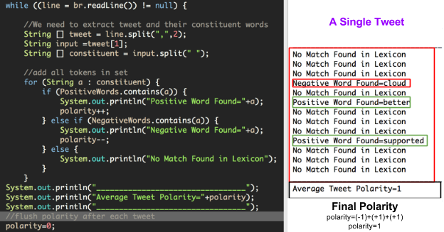
The algorithm has been test driven with less than 30 lines of code, and the output is show below. This is a sample data dump to showcase the inner workings of the algorithm, and the final output file will of course be more concise (i.e. time, polarity format will be obeyed).
As you may have already realized, the world “cloud” and it’s semantics are virtually unknown at this stage, and this is an unsolved problem in NLP called word-sense disambiguation. At this point, we are unable to derive the true meaning and the sense of the word “cloud” which could have multiple meanings, such as cloud computing, the weather cloud or the negative verb. Looking into word-sense disambiguation is beyond the scope of our research project, but it is worth mentioning.
We ran our algorithm on the boeing_improved.txt dataset that we pre-processed earlier. The results are shown on the below. The polarity of a tweet is detectable and the final prediction data point remains to be: date,sentiment (last line).
The output of this algorithm produces company_sentiment.txt, which can be used to plot a time series chart with Y axis representing sentiment and X axis representing time.
This section contains short snippets of the Algorithm 1 implementation. It includes the sentiment polarity calculator along with changing date formats for plotting data on Excel as time series. We also used the SaaS application Plotly to visualize our data.
while ((line = br.readLine()) != null) {
//We need to extract tweet and their constituent words
String [] tweet = line.split(",",3);
String input =tweet[1];
String [] constituent = input.split(" ");
//add all tokens in set
for (String a : constituent) {
if (PositiveWords.contains(a)) {
polarity++;
} else if (NegativeWords.contains(a)) {
polarity--;
} else {
//do nothing literally
}
}
//fix the date and time
SimpleDateFormat sdf = new SimpleDateFormat("EEE/MMM/dd/kk/mm/ss/zzzz/yyyy");
String date = tweet[0].replaceAll(" ","/");
if (date.split("/")[6].length() == 4) {
date = new StringBuilder(date).insert(20, "+").toString();
}
Date d = sdf.parse(date);
String better_date = new SimpleDateFormat("MM/dd/yyyy kk:mm:ss").format(d);
//Let everything be in order again
System.out.println(better_date+","+polarity);
//flush polarity after each tweet
polarity=0;
Results
Boeing’s data has been used to plot a time series data of the tweet sentiment. The data once imported into Excel looks like this (above). The numbers: -1 means negative sentiment, 0 means neutral sentiment and 1 means positive sentiment. Let’s look at the time series plot below.
But before, let’s look at another technique using Logistic Regression.
3.2 Sentiment Analysis using Logistic Regression (via Gradient Descent)
Logistic regression is a simple yet powerful supervised learning algorithm for binary classification. To visualize, the result is a sigmoid which outputs values between 0-1. Since it’s probabilistic, a usual threshold is set to be 0.5.
Features selection
In order to apply this algorithm, the first step is to determine the relevant features which will help mapping tweets to numerical values. We choose to select the 1000th most common words and 1000th most common 2-grams as features.
In other word, each tweet is represented by a vector of 2000 boolean values: if the ith value equals 1, it means than this tweet contains the ith most-common words (if i <= 1000) or the (i-1000)th most common 2-gram (if i > 1000). It worth noticing that the most common words do not include stopwords.
The output we are trying to predict is boolean: it is a binary classification problem. Logistic regression makes use of the sigmoid function to predict whether the tweet should be labeled positive or negative, given the weight parameter theta.
The sigmoid function
Decision boundary: If h(x) >= 0.5 then y = (positive tweet) 1, else y = 0 (negative tweet).
To determine the right weight parameter theta, the algorithm should minimise the cost function of the logistic regression, as shown in the formula below:
- Formula: Cost function of the logistic regression. m is the number of training examples.
The interesting part about Logistic regression is that the function h carries a meaningful information: h(x) is equals to the probability of y being equals to 1 given x.
Implementation: Batch Gradient Descent
Gradient descent is a powerful yet simple way of minimizing a function f. At each iteration of the descent, the algorithm subtracts a part of the gradient of f from the weight vector theta.
Each iteration of the algorithm looks like this:
The speed parameter controls how fast the descent should occur. If the speed is too low, the algorithm will take too much time to converge. If the speed is too high, it is possible to “miss” the local minimum, meaning that the algorithm will diverge. In practice, a speed value of 0.001 performs reasonably well. Note: The full code source of this implementation is available on github: https://github.com/srom/sentiment
Results and observations
The algorithm have been tested on the movie review dataset [6]
The movie review data set is a well known dataset in sentiment analysis. It contains 2000 snippets of movie reviews. The algorithm above performed well, with more than 83% accuracy over the 400 reviews of the test set (20% of the dataset).
4. Correlation with Market Data
Boeing is a DJIA listed company, hence stock data on Yahoo! Finance[3] can give us a good indicator of our sentiment analysis’ correlation with real market data. As our captured data ranges from Jan 1 2014 – Mar 2 2014, it is reasonable to see a snapshot of Boeing’s performance during that time period.
Boeing (Jan 2014 -March 2014) via Y! Finance
In relation to Boeing’s real stock market performance, let us look at a plot generated from our Sentiment Analysis’ Algorithm 1. As you can see below, there seems to be a somewhat resounding correlation of the sentiment analysis for Boeing vs. real stock market data. It would be helpful to have access to yearly Twitter datasets, than quarterly, as it could show better shaped trends. However, towards Feb -March, the data points see a bump and slowly maintain that trend. Let us now look at a standardized plot of Boeing’s sentiment data.
The table below shows the descriptive statistics for our 77000+ data point Boeing sentiment polarity dataset. The mean polarity is 0.1 which is neutral, almost. The data spread is around 0.75 as indicated by the variance. We will now use values of mean and standard deviation to calculate the z-score for each polarity score of a tweet to construct a newer chart.
The plot below shows the time series with z-scores. However, this time, a standard ‘stock market’ bullish/bearish curve has been drawn which makes it easier to understand. The nature of the plot makes it hard to imagine but it correlates closely. For example, towards March, there is a net increase in negative polarity, which would contribute to the sudden downward trend as seen in the real Boeing stock market data obtained from Y! finance earlier.
We have two more datasets that must be put to use, namely amex_improved.txt and att_improved.txt. Let us use Algorithm 1 on them to perform some analysis before we proceed to prediction.
American Express (Data Points > 75,000)
American Express (Jan 2014 - March 2014) via Y! Finance
The overlap of the American Express sentiment data vs. Stock Data using Algorithm 1 shows some very interesting revelations. For example, at around Feb 2014, there is a high net increase in negative polarity, due to some event (we find out later), recorded by tweets alone. This is common, as users vent their anger if a company’s services goes abnormally bad. In correlation, the real stock market data for that period shows the resultant effect a few days later, as visible.
AT&T (Data Points > 1000)
Our final dataset is for AT&T. The image below shows the real stock data chart for AT&T as visible on Y! Finance. If you look closely, there is a sudden drop for AT&T at around Feb 2 – Feb 3, similar to American Express. We have investigated the significance of this time period using Google News and other researching techniques.
The revelation is startling. Since both American Express and AT&T are two highly consumer oriented companies, their stocks went down on Feb 2 2014 – Feb 3 2014. The reason is: SUPERBOWL. The SuperBowl XLVIII[5] was held on 2nd February 2014. Superbowl is America’s most watched event, and people spend more time watching the sport than buying and shopping. But it’s often the boring Superbowl commercials too!
AT&T (Jan 2014 - March 2014) via Y! Finance
5. Prediction of Stock Performance
It is very interesting to predict stock market performance of the companies listed on the Dow Jones Industrial Average purely using Sentiment Analysis. The premise of the idea is to linearly interpolate the values of polarity over the passing of time for prediction purposes.
The sentiment data that was created from our first, sentiment lexicon-driven, approach, using Algorithm 1 has shown much success in our market correlation experiments. However, can it predict how will Boeing’s, American Express’ or AT&T’s perform after March 3rd 2014? Since this report is up to date as of April 28th 2014, it will be easily verifiable, albeit trends do appear over much longer periods of quarters or years.
Predicting Boeing after March 3rd 2014
This is a screenshot (above) of our polarity .txt for Boeing, used in our earlier experiments. The prediction model will have two components, as it is a time series. The X Axis will have the date-time stamps whereas the Y axis will cater to the polarity. The idea is to perform a simple linear regression as we only have a single parameter variable i.e polarity scores of the tweets. The general model for simple linear regression is: y = mx + b.
After conducting a linear regression analysis on our dataset, the Boeing stock is predicted to go up very slightly from March 2nd 2014 onwards, however with Malaysia Airline MH370’s disappearance, Boeing’s stock (in reality) goes down by Mid March onwards. This is a rare scenario which cannot be predicted by sentiment analysis alone. However, Boeing’s stock comes back up again as shown in the Google #BA chart on left. This indicates that given a larger amount of tweet volume, it is somehow possible to predict the long term trend of a company’s stock performance by observing Twitter sentiment. Barring rare scenarios like accidents, the sentiment analysis, in form of our report, forms concrete evidence of why it is a powerful tool for those interested in finance and otherwise, research.
References
[1] “Stopwords.txt – Twitter-sentiment-analysis” – Twitter Sentiment Analysis Using Machine Learning Techniques – Google Project Hosting. Web. 26 Apr. 2014. <https://code.google.com/p/twitter-sentiment-analysis/source/browse/trunk/files/stopwords.txt?r=51>.
[2] “Opinion Mining, Sentiment Analysis, Opinion Extraction.” Opinion Mining, Sentiment Analysis, Opinion Extraction. Web. 27 Apr. 2014. <http://www.cs.uic.edu/~liub/FBS/sentiment-analysis.html#lexicon>.
[3] “Boeing Company (The) Common Sto Stock Chart | BA Interactive Chart – Yahoo! Finance.” Boeing Company (The) Common Sto Stock Chart | BA Interactive Chart – Yahoo! Finance. Web. 27 Apr. 2014. <http://finance.yahoo.com/echarts?s=BA Interactive#symbol=BA;range=1d>.
[4] “Super Bowl XLVIII.” Wikipedia. Wikimedia Foundation, 22 Apr. 2014. Web. 27 Apr. 2014. <http://en.wikipedia.org/wiki/Super_Bowl_XLVIII>.
[5] Json-simple – JSON.simple – A Simple Java Toolkit for JSON – Google Project Hosting.” Json-simple – JSON.simple – A Simple Java Toolkit for JSON – Google Project Hosting. Web. 28 Apr. 2014. <https://code.google.com/p/json-simple/.>.
[6] Movie Review Data – Pang, Lee – 2002 https://www.cs.cornell.edu/people/pabo/movie-review-data/
If you by chance wish to reference this work, you know the deal.
Authors: Ali Gajani, George Ampatzis, Romain Strock
(CS @ UCL 2013-2014)
About Ali Gajani
Hi. I am Ali Gajani. I started Mr. Geek in early 2012 as a result of my growing enthusiasm and passion for technology. I love sharing my knowledge and helping out the community by creating useful, engaging and compelling content. If you want to write for Mr. Geek, just PM me on my Facebook profile.


